THE EMMIX SOFTWARE FOR THE
FITTING OF MIXTURES OF NORMAL
AND t-COMPONENTS

G.J. McLachlan , D. Peel, K.E. Basford*, and P. Adams,

Department of Mathematics,
University of Queensland, St. Lucia,
Queensland 4072, AUSTRALIA

*School of Land and Food,
University of Queensland, St. Lucia,
Queensland 4072, AUSTRALIA

Abstract

We consider the fitting of normal or t-component mixture models to multivariate data, using maximum likelihood via the EM algorithm. This approach requires the initial specification of an initial estimate of the vector of unknown parameters, or equivalently, of an initial classification of the data with respect to the components of the mixture model under fit. We describe an algorithm called EMMIX that automatically undertakes this fitting, including the provision of suitable initial values if not supplied by the user. The EMMIX algorithm has several options, including the option to carry out a resampling-based test for the number of components in the mixture model.

1. INTRODUCTION

Finite mixtures models are being increasingly used to model the distributions of a wide variety of random phenomena. For multivariate data of a continuous nature, attention has focussed on the use of multivariate normal components because of their computational convenience. They can be easily fitted iteratively by maximum likelihood (ML) via the expectation-maximization (EM) algorithm (Dempster, Laird, and Rubin (1977), McLachlan and Krishnan (1997)), as the iterates on the M-step are given in closed form. Also, in cluster analysis where a mixture model-based approach is widely adopted, the clusters in the data are often essentially elliptical in shape, so that it is reasonable to consider fitting mixtures of elliptically symmetric component densities. Within this class of component densities, the multivariate normal density is a convenient choice given its above-mentioned computational tractability.

However, for a set of data containing a group, or groups, of observations with longer than normal tails or atypical observations, the use of normal components may unduly affect the fit of the mixture model. So a more robust approach by modelling the data by a mixture of t distributions is provided. The use of the ECM algorithm to fit this t mixture model is described in McLachlan and Peel (1998).

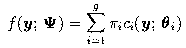
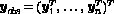
We let y₁,...,y_n denote an observed p-dimensional sample of size n. With a mixture model-based approach to drawing inferences from these data, each data point is assumed to be a realization of the random p-dimensional vector Y with the g-component mixture probability density function (p.d.f.),

where the mixing proportions are nonnegative and sum to one and 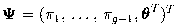where denotes the unknown parameters of the distribution of c_i. In the case of multivariate normal mixture models the are replaced by denoting the multivariate normal p.d.f. with mean (vector) and covariance matrix . Hence the contains the elements of the and the distinct elements of (i=1,...,g). Often, in order to reduce the number of unknown parameters, the component-covariance matrices are restricted to being equal, or even diagonal as in the AutoClass program of Cheeseman and Stutz (1996). Less restrictive constraints can be imposed by a reparameterization of the component-covariance matrices in terms of their eigenvalue decompositions as, for example, in Banfield and Raftery (1993). In the latest version of (AutoClass C ), the covariance matrices are unrestricted In other software for the fitting of mixture models, there are MCLUST and EMCLUST which are a suite of S-PLUS functions for hierarchical clustering EM, and BIC, respectively based on parameterized Gaussian mixture models; see Banfield and Raftery (1993), Byers and Raftery (1998), Campbell et al. (1998), DasGupta and Raftery (1998), and Fraley and Raftery (1998). MCLUST and EMCLUST are written in FORTRAN with an interface to the S-PLUS commercial package. Some packages for the fitting of finite mixtures have been reviewed recently by Haughton (1997). Also, Wallace and Dowe (1994) have considered the application of their SNOB program to mixture modelling using the minimum message length principle of Wallace and Boulton (1968). More recently, Hunt and Jorgensen (1997) have developed the MULTIMIX program for the fitting of mixture models to data sets that contain categorical and continuous variables and that may have missing values.

Under the assumption that y₁,...,y_n are independent realizations of the feature vector Y, the log likelihood function for is given by

With the maximum likelihood approach to the estimation of , an estimate is provided by an appropriate root of the likelihood equation,

In this paper, we describe an algorithm called EMMIX that has been developed using the EM algorithm to find solutions of (1.3) corresponding to local maxima. In the appendix of their monograph, McLachlan and Basford (1988) gave the listing of FORTRAN programs that they had written for the maximum likelihood fitting of multivariate normal mixture models under a variety of experimental conditions. Over the years, these programs have undergone continued refinement and development, leading to an interim version known as the NMM algorithm (McLachlan and Peel, 1996). Since then, there has been much further development, culminating in the present version of the algorithm known as EMMIX . The option in EMMIX that uses hierarchical-based methods for the provision of an initial classification of the data uses the the program HACLUS written by Dr I. De Lacy.

For the mixture programs of McLachlan and Basford (1988), an initial specification had to be given by the user either for the parameter vector or for the classification of the data with respect to the components of the normal mixture model. With the EMMIX algorithm, the user does not have to provide this specification. In the absence of a user-provided specification, the EMMIX algorithm can be run for a specified number of random starts and/or for starts corresponding to classifications of the data by specified clustering procedures from a wide class that includes k-means and commonly used hierarchical methods.

Another major option of the EMMIX algorithm allows the user to automatically carry out a test for the smallest number of components compatible with the data. This likelihood-based test uses the resampling approach of McLachlan (1987) to assess the associated P -value. This option is based on the MMRESAMP subroutine of McLachlan et al. (1995). The EMMIX algorithm also has several other options which are outlined in the user's guide.

2. APPLICATION OF EM ALGORITHM

It is straightforward to find solutions of (0.3) using the EM algorithm of Dempster et al. (1977). For the purpose of the application of the EM algorithm, the observed-data vector is regarded as being incomplete. The component-label variables are consequently introduced, where is defined to be one or zero according to if did or did not arise from the i th component of the mixture model, (i=1, ... ,g; j=1,...,n). This complete-data framework in which each observation is conceptualized as having arisen from one of the components of the mixture is directly applicable in those situations where Y can be physically identified as having come from a population which is a mixture of g groups. On putting 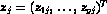, the complete-data vector is therefore given by

where are taken to be independent and identically distributed with z₁,...,z_n being independent realizations from a multinomial distribution consisting of one draw on g categories with respective probabilities . That is,

where .

For this specification, the complete-data log likelihood is

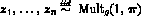
The EM algorithm is easy to program and proceeds iteratively in two steps, E (for expectation) and M (for maximization); see McLachlan and Krishnan (1997) for a recent account of the EM algorithm in a general context. On the (K+1) th iteration, the E-step requires the calculation of

the conditional expectation of the complete-data log likelihood , given the observed data , using the current fit for . Since is a linear function of the unobservable component-label variables , the E-step is effected simply by replacing by its conditional expectation given , using for . That is, is replaced by

where is the current estimate of the posterior probability that the j th entity with feature vector belongs to the i th component, (i=1,...,g; j=1,...,n).

On the M-step on the (k+1) th iteration, the intent is to choose the value of , say , that maximizes . It follows that on the M-step of the (k+1) th iteration, the current fit for the mixing proportions, the component means, and the covariance matrices is given explicitly by

and

for i=1,...,g.

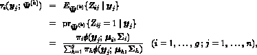
A nice feature of the EM algorithm is that the mixture likelihood can never be decreased after the EM sequence. Hence

which implies that converges to some L* for a sequence of likelihood values bounded above. The E and M-steps are alternated repeatedly until the likelihood (or the parameter estimates) change by an arbitrarily small amount in the case of convergence.

Let be the chosen solution of the likelihood equation. The likelihood function tends to have multiple local maxima for normal mixture models. In this case of unrestricted component covariance matrices, is unbounded, as each data point gives rise to a singularity on the edge of the parameter space; see, for example, McLachlan and Basford (1988, Chapter 2). In practice, however, consideration has to be given to the problem of relatively large local maxima that occur as a consequence of a fitted component having a very small (but nonzero) variance for univariate data or generalized variance (the determinant of the covariance matrix) for multivariate data. Such a component corresponds to a cluster containing a few data points either relatively close together or almost lying in a lower dimensional subspace in the case of multivariate data. There is thus a need to monitor the relative size of the fitted mixing proportions and of the component variances for univariate observations and of the generalized component variances for multivariate data in an attempt to identify these spurious local maximizers. There is also a need to monitor the Euclidean distances between the fitted component means to see if the implied clusters represent a real separation between the means or whether they arise because one or more of the clusters fall almost in a subspace of the original feature space.

3. MIXTURES OF t-DISTRIBUTIONS

As mentioned in Section 2, for many applied problems, the tails of the normal distribution are often shorter than required. Also, the estimates of the component means and covariance matrices can be affected by observations that are atypical of the components in the normal mixture model being fitted. EMMIX provides a more robust approach by modelling the data by a mixture of t distributions. The use of the ECM algorithm to fit this t mixture model is described and examples of its use are given in McLachlan and Peel(1998). With this t mixture model-based approach, the normal distribution for each component in the mixture is embedded in a wider class of elliptically symmetric distributions with an additional parameter called the degrees of freedom

. As

tends to infinity, the t distribution approaches the normal distribution. Hence this parameter

may be viewed as a robustness tuning parameter. EMMIX has the option to fix the component

parameters in advance or infer their values from the data for each component using the ECM algorithm.

4. SPECIFICATION OF INITIAL VALUES

It follows from above that care must be taken in the choice of the root of the likelihood equation in the case of unrestricted covariance matrices where is unbounded. In order to fit a mixture model using the EM algorithm, an initial value has to be specified for the vector of unknown parameters for use on the E-step on the first iteration of the EM algorithm. Equivalently, initial values must be specified for the posterior probabilities of component membership of the mixture, 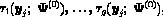, for each for use on commencing the EM algorithm on the M-step the first time through. The latter posterior probabilities can be specified as zero-one values, corresponding to an outright classification of the data with respect to the g components of the mixture. In this case, it suffices to specify the initial partition of the data. In a cluster analysis context it is usually more appropriate to do this rather than specifying an initial value for .

5. EMMIX ALGORITHM

We now give a general description of an algorithm called EMMIX, which automatically provides a selection of starting values for this purpose if not provided by the user. More precise details on the EMMIX algorithm, including its implementation, are given in the ``User's Guide to EMMIX''.

The EMMIX algorithm automatically provides starting values for the application of the EM algorithm by considering a selection obtained from three sources:

(a) random starts,
(b) hierarchical clustering-based starts, and
(c) k-means clustering-based starts

Concerning (a) for randomly selected starts, we have an additional option whereby the user can first subsample the data before using a random start based on the subsample each time. This is to limit the effect of the central limit theorem which would have the randomly selected starts being similar for each component in large samples.

Concerning (b), the user has the option of using in either standardized or unstandardized form, the results from seven hierarchical methods (nearest neighbour, farthest neighbour, group average, median, centroid, flexible sorting, and Ward's method). There are several algorithm parameters that the user can optionally specify; alternatively, default values are used. The program fits the normal mixture model for each of the initial grouping specified from the three sources (a) to (c). All these computations are automatically carried out by the program. The user only has to provide the data set the restrictions on the component-covariance matrices (equal, unequal, or diagonal), the extent of the selection of the initial groupings to be used to determine starting values, and the number of components that are to be fitted. Summary information is automatically given as output for the final fit. However, it is not suggested that the clustering of a data set should be based solely on a single solution of the likelihood equation, but rather on the various solutions considered collectively. The default final fit is taken to be the one corresponding to the largest of the local maxima located. However, the summary information can be recovered for any distinct fit.

As well as the options pertaining to the automatic provision of starting values covered above, several other options are available, including the provision of standard errors for the fitted parameters in the mixture model, and the bootstrapping of the likelihood ratio statistic for testing versus components in the mixture model, where the value is specified by the user. With the latter option, the bootstrap samples are generated parametrically from the -component normal mixture model with set equal to the fit for under the null hypothesis of components.

6. EXAMPLE

To illustrate the use of the EMMIX algorithm, we consider a simulated bivariate sample generated from a normal mixture model with parameters

means=[0 0],[4 0],[-4 0] and
covariances= [1 0] [1   -.4] [2  .3]
             [0 1] [-.4   3] [.3 .5]

A plot of the sample with the true allocation shown is given in Figure 1.

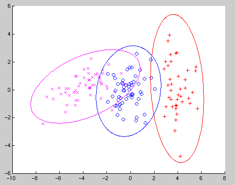
Figure 1: Plot of the simulated sample with the true allocation shown

We now cluster these data, ignoring the known classification of the data, by fitting a mixture of three normal components with 10 random starts (using 70% subsampling of the data), 10 k-means starts and the default 6 hierarchical methods (with and without restrictions on the component-covariance matrices). The resulting allocation when fitting unconstrained covariance matrices is shown in Figure 2.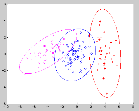

Figure 2: Plot of the allocation found by EMMIX with arbitrary covariance matrices for the simulated sample

When fitting unconstrained covariance matrices EMMIX misallocated eight points (5.3 %). The misallocations occur on the boundary between the purple and blue groups, with EMMIX misallocating seven of the purple group as blue and one of the blue points purple.

Similarly, the allocation produced when fitting equal covariance matrices is given in Figure 3. Fitting equal covariance matrices in this example results, as would be expected, in a much larger number of misallocations.

Figure 2: Plot of the allocation found by EMMIX with equal covariance matrices for the simulated sample

If the number of components is not specified, EMMIX can fit a range of values for the number of components utilizing the bootstrap procedure. The resulting output from EMMIX (fitting unconstrained covariance matrices) is given below in Table 1.

 -------------------------------------------------------------------------
 | NG | Log Lik | -2log(lambda) |   AIC   |   BIC   |   AWE   | P-value  |
 -------------------------------------------------------------------------
 |  1 | -636.76 |      -        | 1283.53 | 1298.58 | 1333.64 |    -     |
 -------------------------------------------------------------------------
 |  2 | -612.31 |     48.92     | 1246.61 | 1279.73 | 1356.85 |   0.01   |
 -------------------------------------------------------------------------
 |  3 | -588.21 |     48.19     | 1210.42 | 1261.60 | 1380.78 |   0.01   |
 ------------------------------------------------------------------------
 |  4 | -580.79 |     14.84     | 1207.58 | 1276.82 | 1438.07 |   0.12   |
 -------------------------------------------------------------------------

Table 1: Analysis to determine the number of groups for the simulated example

The results produced by EMMIX shown in Table 1 concur with the true number of components, three.

REFERENCES

Banfield, J.D., and Raftery, A. (1993). Model-based Gaussian and non-Gaussian clustering. Biometrics 49, 803-821.

Byers, S. and Raftery, A.E. (1988). Nearest-neighbor clutter removal for estimating features in spatial point processes. Journal of the American Statistical Association 91, 577-584.

Campbell, J.G., Fraley, C., Murtagh, F., and and Raftery, A.E. (1998). Linear flaw detection in woven textiles using model-based clustering. Pattern Recognition Letters 18, 1539-1548.

Cheeseman, P., and Stutz, J. (1996). Bayesian classification (AutoClass): theory and results. In Advances in Knowledge Discovery and Data Mining , U.M. Fayyad, G. Piatetsky-Shapiro, P. Smyth, and R. Uthurusamy (Eds.). Menlo Park, California: The AAAI Press, pp. 61-83.

DasGupta, A. and Raftery, A.E. (1998). Detecting features in spatial point processes with clutter via model-based clustering. Journal of the American Statistical Association 93, 294-302.

Dempster, A.P., Laird, N.M., and and Rubin, D.B. (1997). Maximum likelihood from incomplete data via the EM algorithm (with discussion). Journal of the Royal Statistical Society B 39, 1-38.

Fraley, C. and Raftery, A.E. (1998). How many clusters? Which clustering method? - Answers via model-based cluster analysis. Technical Report No. 329. Seattle: Department of Statistics, University of Washington.

Hastie, T. and Tibshirani, R.J. (1996). Discriminant analysis by Gaussian mixtures. Journal of the Royal Statistical Society B 58, 155-176.

Haughton, D. (1997). Packages for estimating finite mixtures: a review. Applied Statistics 51, 194-205.

Hunt, L., and Jorgensen, J. (1997). Mixture model clustering: a brief introduction to the MULTIMIX program. Unpublished manuscript.

McLachlan, G.J. (1987). On bootstrapping the likelihood ratio test statistic for the number of components in a normal mixture. Applied Statistics 36, 318-324.

McLachlan, G.J. and Basford, K.E. (1988). Mixture Models: Inference and Applications to Clustering . New York: Marcel Dekker.

McLachlan, G.J. and Krishnan, T. (1997). The EM Algorithm and Extensions . New York: Wiley.

McLachlan, G.J. and Peel, D. (1996). An algorithm for unsupervised learning via normal mixture models. In ISIS: Information, Statistics and Induction in Science , D.L. Dowe, K.B. Korb, and J.J. Oliver (Eds.), pp. 354-363. Singapore: World Scientific.

McLachlan, G.J., Peel D., Adams, P., and Basford, K.E. (1995). An algorithm for assessing by resampling the P-value of the likelihood ratio test on the number of components in normal mixture models. Research Report No. 31 . Brisbane: Centre for Statistics, The University of Queensland.

McLachlan, G.J. and Peel, D. (1998). Robust cluster analysis via mixtures of multivariate t-distributions. In Lecture Notes in Computer Science Vol. 1451, A. Amin, D. Dori, P. Pudil, and H. Freeman (Eds.). Berlin: Springer-Verlag, pp. 658-666.

Wallace, C.S and Boulton, D.M. (1968). An information measure for classification. Computer Journal 11, 185-194.

Wallace, C.S. and Dowe D.L. (1994). Intrinsic classification by MML - the Snob program. In 7th Australian Joint Conference on Artificial Intelligence, 37-44.

THE EMMIX SOFTWARE FOR THE FITTING OF MIXTURES OF NORMAL AND t-COMPONENTS