MODELLING QUASISTATIONARITY IN EVANESCENT PROCESSES
by
Phil Pollett
Department of Mathematics
The University of Queensland
(Download the following image (as postscript)):

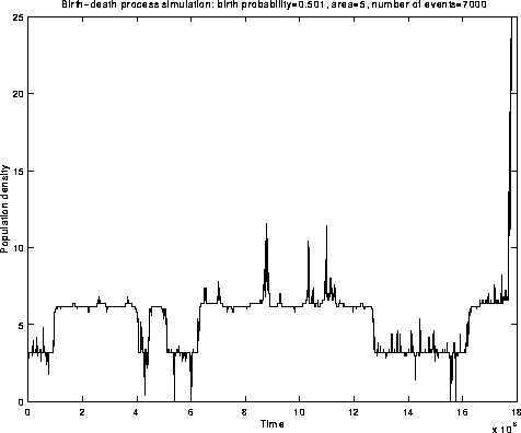
Figure 1. Quasistationarity of an explosive population process
[Simulation |
java code]
QUASISTATIONARITY
Processes appear to be stationary over any reasonable time scale, yet they are evanescent.
Examples:
AN AUTO-CATALYTIC REACTION
Consider the following reaction scheme:

where X is a catalyst. Suppose that there are two stages, namely

Let  number of X molecules at time t.
Suppose that the concentration of A is held constant;
let a be the number of molecules of A.
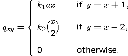
The state space is  and the transition rates,
  , are given by
(Download the following image (as postscript)):
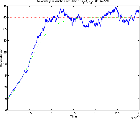
Figure 2. Auto-catalytic reaction simulation
[Simulation |
java code]
AN EPIDEMIC MODEL
(Ridler-Rowe)
The state at time t:
 - number of susceptibles
 - number of infectives
State space:

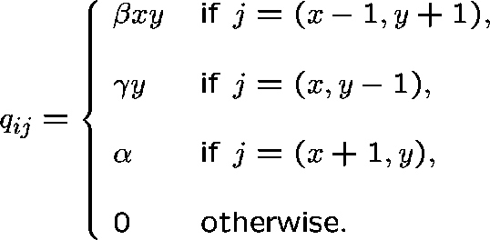
Transition rates  :
:
if  , then
(Download the following image (as postscript)):
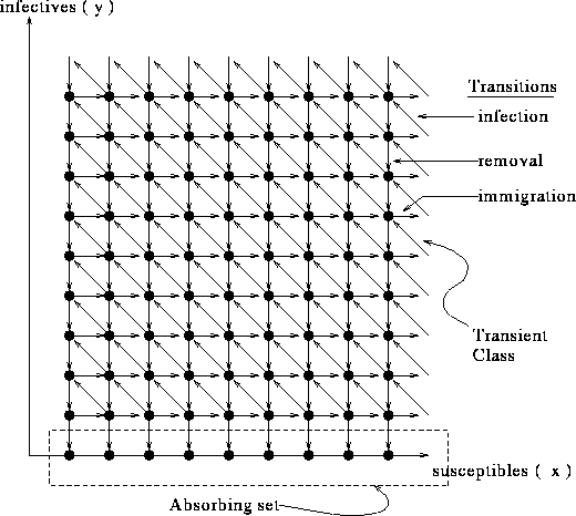
Figure 3. State transition diagram for
Ridler-Rowe epidemic model.
Clearly,

is an irreducible transient class.
Ridler-Rowe (1967): Q is regular (nonexplosive) and absorption occurs with probability 1.
(Download the following image (as postscript)):
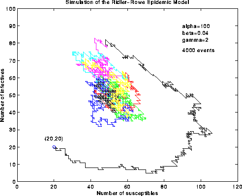
Figure 4. Simulation of the Ridler-Rowe epidemic model
[Simulation |
java code]
(Download the following image (as postscript)):
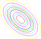
Figure 5. Simple contour plot of the usual diffusion
approximation for the Ridler-Rowe epidemic model
(to be imagined as superimposed on Figure 4)
(Download the following image (as postscript)):
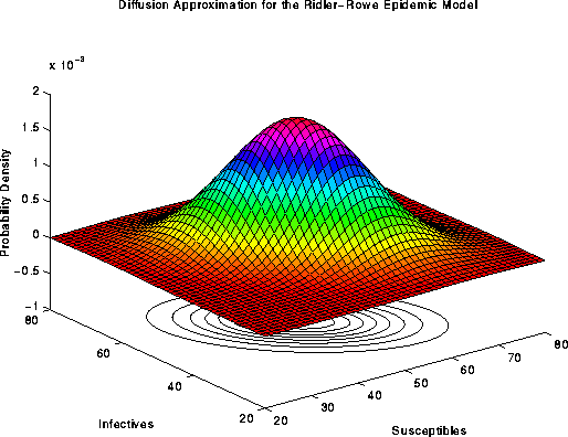
Figure 6. Surface plot of the usual diffusion
approximation for the Ridler-Rowe epidemic model
QUASISTATIONARY DISTRIBUTIONS
Notation. Let  be the state of the system at time t and
suppose that
  , where S, the state space, is a discrete
set. Let
  be the matrix of transition rates
(q-matrix), so that
  , for
, for  , represents
the transition rate from state i to state j and
  ,
where
  represents the transition
rate out of state i.
Assumptions. Take 0 to be the sole absorbing state, that is,
 , and suppose that
  , where
  is an irreducible class. In order that there be a positive probability
of ever reaching 0, given that the process starts in C, suppose that
 for at least one
  .
.
Let  ,
,  .
.
Definition.
Let  be a probability distribution over C and let

Then,  is a quasistationary distribution
if

That is, if the process has  as its initial distribution, then
  is a
quasistationary distribution
if the state probabilities at time t, conditional on the process
being in C at t, are the same for all t.
If  is a quasistationary distribution
then, under certain conditions,

no matter what the value of  .
.
A CHARACTERIZATION
If  is a quasistationary distribution,
then clearly

where  .
It is easy to show that g satisfies:

and  .
Thus,
  , for some
  .
Since the converse is also true,
we have the following result:
Proposition.
A probability distribution,  , over C
is a quasistationary distribution
if and only if, for some
  ,
,  is a
is a  -invariant
measure, that is

HOW DO WE DETERMINE  from Q?
Rewrite (1) as

and remember that
 is the right-hand derivative of
  near 0.
So, on dividing by t and letting
  , we get (formally)

or, equivalently,

Accordingly, we shall say that  is a
is a  -invariant measure for
Q whenever (2) holds.
Proposition.
If  is a quasistationary distribution
then, for some
  ,
,  is a
is a  -invariant
measure for Q.
IS THE CONVERSE TRUE?
Suppose that, for some  ,
,  is a
is a  -invariant measure for
Q, that is

Is  a quasistationary distribution?
Sum this equation over  :
we get (formally)


Theorem.
Let  be a probability distribution
over C
and suppose that
  is a
is a  -invariant measure
for Q. Then,
 with equality if and only if
  is a quasistationary distribution.
AN EXAMPLE
The birth-death-catastrophe process.
Let  and suppose that

where  , a>0,
 for at least one value of
  and
and
 .
Thus, jumps occur at a constant ``per capita'' rate
  and,
at a jump time, a birth occurs with probability a, or
otherwise a catastrophe occurs, the size of which is determined by
the probabilities
  ,
,  .
.
Clearly, 0 is an absorbing state and
 is an irreducible class.
So, does the process admit a quasistationary distribution?
Substitute the transition rates in (2):

and, for  ,
,

If we try a solution of the form  , the first equation tells us
that
  , where

and, on substituting both of
these quantities in the second equation, we find that  .
This latter equation has a unique solution,
  , on
, on  .
Thus, by setting
  we can obtain a positive solution,
 , to (2), such that
  whenever
  . Further, it is easy to
show that
  .
.
The condition  is satisfied only in the subcritical case,
that is, when the drift, D, given by

is strictly negative; incidentally, this also guarantees that absorption occurs with probability 1.
Proposition.
The subcritical birth-death-catastrophe process has a
geometric quasistationary distribution
,  , given by

where  is the unique solution to
  on the
interval
  .
.
COMPUTATIONAL METHODS
Finite S : Mandl (1960) showed that the restriction of Q to
C has eigenvalues with negative real parts and the one with maximal
real part (called  above) is real and has multiplicity 1, and,
the corresponding left eigenvector,
  , has positive
entries; this is, of course, a
  -invariant measure for Q (unique
up to constant multiples). Since S is finite, the quasistationary distribution,
 , exists and is given by

Infinite S : Truncate the restriction of Q to an  matrix,
  , and construct a sequence,
  , of
eigenvectors and hope that this converges to a
  -invariant measure, m,
for Q, et cetera.
HOW SHOULD WE EVALUATE m?
Consider the Ridler-Rowe epidemic model.
First truncate C to

and restrict Q to  .
Use the transformation
 to convert the restricted q-matrix into an
  matrix,
  , where
  .
.
Evaluation of the eigenvectors of Q is not completely
trivial. For example, if (as well shall assume) N=100,
that is  , Q needs 400 Mbytes of storage.
However, for N large, this matrix is large and sparse. Does this help?
THE ARNOLDI METHOD
We need to solve  , where
  .
.
Using an initial estimate of x, the basic Arnoldi method produces an
 (upper-Hessenberg) matrix
  and an
 matrix
  with
with

and such that if  is an eigenvector of
 , then, for m large,
  is close
to an eigenvector of A.
Solve for  using standard (dense-matrix) methods.
AN ITERATIVE ARNOLDI METHOD
Take m small (we found that m=20 worked best).
Then,
using an initial estimate,  , of the eigenvector x,
apply the basic Arnoldi method (to obtain
  and
and  ) and
set
  to be the dominant eigenvalue of
  if this is real, or set
  equal to zero otherwise.
Now solve

with z chosen at random and repeat the procedure with a new initial estimate, given by

Continue until the residual,  , is
sufficiently small.
(Download the following image (as postscript)):
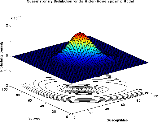
Figure 7. Surface plot of the quasistationary distribution
for the Ridler-Rowe epidemic model
(Download the following image (as postscript)):
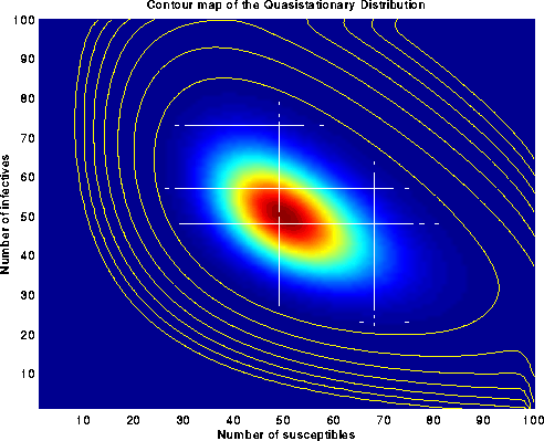
Figure 8. Contour plot of the quasistationary distribution
for the Ridler-Rowe epidemic model
(Download the following image (as postscript)):
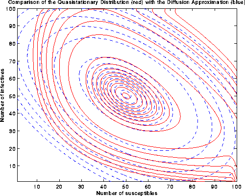
Figure 8. Comparison between the quasistationary distribution
and the diffusion approximation (contour plot) for the
Ridler-Rowe epidemic model
(Download the following image (as postscript)):
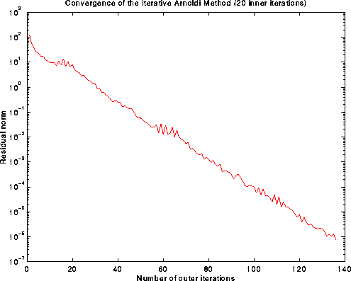
Figure 10. Graph of the residual norm versus the
number of outer iterations for the
Iterative Arnoldi Method
(Download the following image (as postscript)):
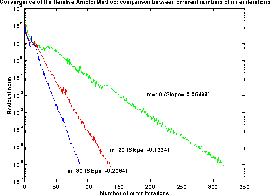
Figure 11. Graph of the residual norm versus the
number of outer iterations for various
values of m, the number of inner iterations