LIMITING CONDITIONAL DISTRIBUTIONS FOR STOCHASTIC METAPOPULATION MODELS
by
Phil Pollett
Department of Mathematics
The University of Queensland
CONDITIONAL STATE DISTRIBUTION
X(t) - state of the population at time t
We suppose thatis a continuous time Markov chain with a discrete state space
, where 0 is the state corresponding to extinction and
comprises the remaining states.
![]() - state probabilities
- state probabilities
We observe the population at an arbitrary time u and extinction has not yet occurred. How can we incorporate this information?
The conditional state distribution
Evaluate the state probabilities at time u conditioned on non-extinction:

A STOCHASTIC MODEL FOR METAPOPULATIONS
There are n geographical regions (patches):
 Let
Let ![]() ,
where
,
where ![]() is 1 or 0 according as patch i is
occupied or not at time t (
is 1 or 0 according as patch i is
occupied or not at time t ( ![]() ).
Note that the state space is
).
Note that the state space is ![]() .
.
 - Interaction matrix:
, for
, is the probability that patch j will not be colonized by migration from patch i, and
is the probability that (in the absence of immigration) patch i will become extinct.
Assume (Gyllenberg and Silvestrov) that
![]()
where ![]() is the distance between patches i
and j (
is the distance between patches i
and j ( ![]() and
and ![]() ),
),
![]() is the area of patch i
and a(
is the area of patch i
and a( ![]() ) measures how badly individuals are at migrating.
) measures how badly individuals are at migrating.
THE TRANSITION PROBABILITIES
Assume that the various colonization processes and local extinction
processes are independent. Define ![]() , where
, where
![]() , by
, by

to be the probability that patch j will become extinct at the next epoch given a present configuration x.
The transition matrix ![]()

Note that, since ![]() ,
,  , state
 ![]() (corresponding to the extinction of all patches) is an absorbing state
for the chain:
(corresponding to the extinction of all patches) is an absorbing state
for the chain:

A 5-PATCH METAPOPULATION

Patches 2, 3, 4 & 5 are equally
spaced (a distance 0.1 apart), while Patch 1 is 10 times that distance away
from the others ( ![]() ).
All patches have the same area.
).
All patches have the same area.
PERSISTENCE OF METAPOPULATIONS: QUASI-STATIONARITY
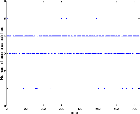
Simulation of the 5-patch model with a=7. The number of occupied patches is plotted against time (up to extinction at t=728).
Do the conditional state probabilities account for the observed behaviour?
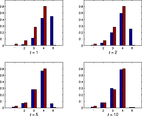
Comparison of the observed frequencies with the conditional state
distribution ![]() at t=1,2,5,10.
The brown
bar is the proportion of time for which i patches were occupied
(
at t=1,2,5,10.
The brown
bar is the proportion of time for which i patches were occupied
( ![]() ) during the period of the simulation.
The blue bar is the distribution
of the number of occupied patches evaluated using
) during the period of the simulation.
The blue bar is the distribution
of the number of occupied patches evaluated using ![]() .
.
LIMITING CONDITIONAL DISTRIBUTIONS
The observed trend has a simple theoretical
explanation. Since ![]() is a finite set, the limit
is a finite set, the limit
![]()
exists and defines a proper distribution ![]() , called a
limiting conditional distribution, and m is the left
eigenvector of
, called a
limiting conditional distribution, and m is the left
eigenvector of ![]() (P restricted to
(P restricted to ![]() ) corresponding to the
eigenvalue,
) corresponding to the
eigenvalue, ![]() , with maximal modulus
(Darroch and Seneta (1965)).
Note that the expected time till absorption,
, with maximal modulus
(Darroch and Seneta (1965)).
Note that the expected time till absorption, ![]() , is approximately
, is approximately
![]() .
.
We can be precise about the rate of
convergence by examining the eigenvalue, ![]() , of
, of
![]() with second-largest modulus. It might not
be real, and it has multiplicity
with second-largest modulus. It might not
be real, and it has multiplicity ![]() (for simplicity, suppose
(for simplicity, suppose ![]() ). It can be
shown that
). It can be
shown that
![]()
where ![]() .
.
THE CONVERGENCE OF ![]() TO
TO ![]()
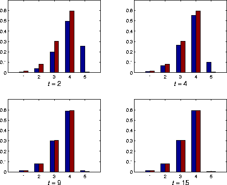
Comparison between the conditional state distribution (blue) and the limiting conditional distribution (brown) of the number of occupied patches for the 5-patch metapopulation model with a=7.
For the 5-patch metapopulation model with a=7, we
find that ![]() ,
, ![]() (real with
multiplicity 1),
(real with
multiplicity 1), ![]() and
and ![]() .
.
PSEUDO-STATIONARY DISTRIBUTIONS
(The method of Gyllenberg and Silvestrov)
Rationale: If we had assumed that Patch 1 (say) had
a zero local extinction probability ( ![]() ), that patch would
behave as a mainland. State 0 would no
longer be accessible from all states:
), that patch would
behave as a mainland. State 0 would no
longer be accessible from all states: ![]() would decompose
into two classes,
would decompose
into two classes, ![]() and
and ![]() , consisting of those
states in
, consisting of those
states in ![]() which have
which have ![]() and
and ![]() respectively; either the
process would start in
respectively; either the
process would start in ![]() (mainland inhabited) and remain
there, or, start in
(mainland inhabited) and remain
there, or, start in ![]() (mainland uninhabited) and eventually
enter either
(mainland uninhabited) and eventually
enter either ![]() or the absorbing state.
or the absorbing state.
We identify a ``quasi-mainland'', namely a single patch i
with ![]() small (say Patch 1), and consider a sequence of
processes indexed by
small (say Patch 1), and consider a sequence of
processes indexed by ![]() , treating
, treating ![]() as a
perturbation.
as a
perturbation.
PERTURBATION THEORY
Let ![]() (now arbitrary) and suppose that our interaction
matrix depends on
(now arbitrary) and suppose that our interaction
matrix depends on ![]() in the following way:
in the following way:

where

the latter assumed to be non-negative and finite, and, that  satisfies
 ![]() .
.
Then, in an obvious notation,
![]()
where  is the
transition matrix corresponding to
  and
and ![]() is the transition matrix corresponding to Q.
is the transition matrix corresponding to Q.
THE G&S LIMITING REGIME
Let ![]() and
and ![]() in such a way that
in such a way that
![]() , where
, where ![]() .
Since the expected lifetime of the
quasi-mainland is of order
.
Since the expected lifetime of the
quasi-mainland is of order ![]() , one is able to study the
process on different time scales
(s=0,
, one is able to study the
process on different time scales
(s=0, ![]() , and
, and ![]() ).
).
G&S showed that the limit
![]()
exists and is given by a mixture of the limiting probabilities
![]() for the (ergodic) chain generated by Q and the degenerate
distribution
for the (ergodic) chain generated by Q and the degenerate
distribution ![]() which assigns all its mass to state 0, the
mixing probability being
which assigns all its mass to state 0, the
mixing probability being ![]() , where
, where ![]() is a positive
constant which is specified in terms of
is a positive
constant which is specified in terms of ![]() .
.
A COMPARISON USING THE 5-PATCH MODEL
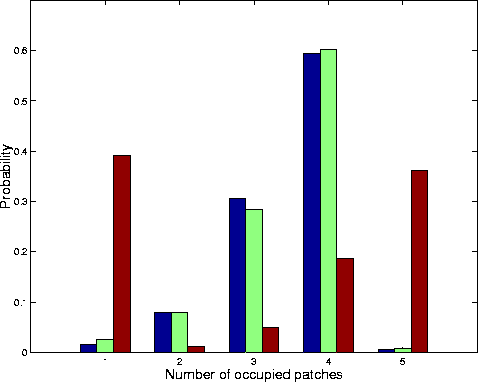
Comparison between the limiting conditional distribution (blue), the simulated proportions (green) and the pseudo-stationary distribution (brown).
The disparity is marked: for this example, the two ways of analysing the model lead to quite different predictions.
THE EFFECT OF VARYING s
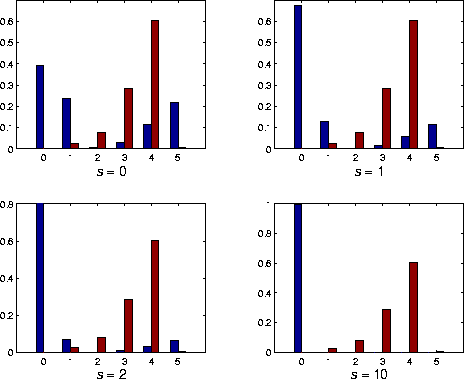
The effect of varying s on the pseudo-stationary distribution (blue). The brown bar represents the simulated proportions of occupied patches.
Observe that the disparity becomes worse as the time-scale parameter s increases.
RECONCILIATION
Denote the state probabilities corresponding to ![]() by
by
 ,
and denote the corresponding conditonal probabilities by
 . Gosselin (1997) proved that

which he compared with Theorem 6.2 of G&S:

Thus, in the important case
s=0, the limiting conditonal distribution and the pseudo-stationary
agree when ![]() is small.
is small.
The problem with the 5-patch model is that ![]() - not sufficiently small.
- not sufficiently small.
REMARKS
Quasi-stationarity is a property of the model
and not the means of analysing it. The 5-patch model exhibits
quasi-stationarity, demonstrated emphatically using simulation, yet
![]() is not small. The pseudo-stationary distribution does not
capture this behaviour. On the other hand, the conditional state
distribution m(t) does: afterall, it is the most information our
model can provide at any time t given that we know extinction has
not occured by time t. In cases when the convergence of m(t) to the
limiting conditional distribution m is rapid, this
distribution can be used instead.
is not small. The pseudo-stationary distribution does not
capture this behaviour. On the other hand, the conditional state
distribution m(t) does: afterall, it is the most information our
model can provide at any time t given that we know extinction has
not occured by time t. In cases when the convergence of m(t) to the
limiting conditional distribution m is rapid, this
distribution can be used instead.